Dynamic Named Ranges

The power of Dynamic Named Ranges cannot be underestimated. They allow a calculation or list of information to be updated automatically when information is added or deleted. I mostly use them when creating validation listboxes but they can alos be used very effectively in formulas and graph source data.
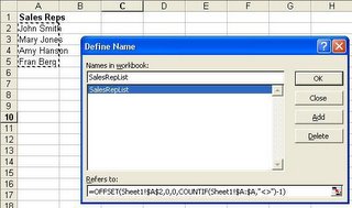
In order to create a dynamic Named Range it is necessary to utilise the 'offset' function in the 'Refers to' textbox in the Define Name dialog box.
Example - dynamic Named Range

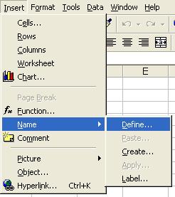
1. Insert Menu - > Name -> Define





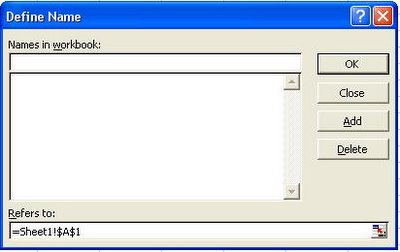
2. This will bring up the Define Name dialog





3. Enter the name you wish to call your Named Range in the Names in workbook textbox
   


4. In the refers to textbox, enter the following formula




=OFFSET(Sheet1!$A$2,0,0,COUNTIF(Sheet1!$A:$A,"<>")-1)





Information about the formula/function



• From cell A2, select all cells in column A that are not blank minus 1 (to exclude the heading)


• You could substitute "<>" for ">0" (greater than 0) or any other criteria you chose.


• If you delete or enter another name from the list then the Named Range will automatically include it in the selection



Where this could be used



• In a formula


• Data validation 'List'


• Chart Source information - for example, it is March, so only 3 months of Sales have been recorded but unless you change the source selection of the chart each month, the graph will show all the months up to December (even though they haven't occurred yet). Why not enter a Named Range as the Source data so that it automatically picks up the 'current' sales (up to and including March)

Named Ranges

a very nice feature of Excel is the ability to create named ranges so that cell references or even values can be given a more meaningful definition.
Creating a Named Range

1. To create a named range simply go to the Insert Menu - > Name -> Define
2. This will bring up the Define Name dialog
3. Enter a name in the Names in workbook textbox
4. In the refers to textbox you can enter a the following pieces of information:
• Ranges ($A$1:$A$5)
• Values (10% - could be used for the named range GST)
5. Click the 'Add' button and then 'OK'

Example 1 - create a named range for a range of cells

1. Insert Menu - > Name -> Define





2. This will bring up the Define Name dialog





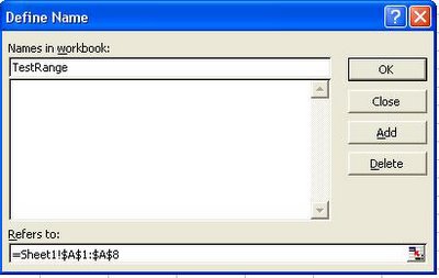
3. Enter TestRange in the Names in workbook textbox





4. In the refers to textbox, select range A1 to A8 of Sheet 1


5. You can now use this in a formula for example, =Sum(TestRange), will total the values in cells A1:A8 of Sheet1

Example 2 - create a named range for a value

1. Insert Menu - > Name -> Define





2. This will bring up the Define Name dialog





3. Enter GST in the Names in workbook textbox
4. In the refers to textbox, enter =10%





5. You can now use this in a formula for example, =A1*GST, will multiply the value in cell A1 by 10%

Layout Layout Layout!

The most important thing in creating and setting up a Microsoft Excel workbook is correctly laying out the sheets in a respectable manner. Generally, with the majority of my workbooks I have 4 sheets for a set of data. 'Overview', 'Data', 'Summary' and 'Graphs'. For the purpose of this topic I have used an example

Overview
This sheet contains an overview of what is contained in the workbook and 3 hyperlinks to the other 3 sheets outlined below. View an example
Data
This sheet contains the table of information. This sheets should be laid out so that headings are in row 1 in bold and there are no blank rows of data, otherwise Excel will no consider any data below the blank row a part of the 'current' dataset. View an example
Summary
The summary sheets contains the information that you wish to analyse; it may be the total sales by month by Sales Rep.. I always like to have the months running down the rows and the other category (Sales Rep. for example) running across the columns. This is because there are at least 12 months that you wish to analyse and generally it is easier to read more than 8 categories downward. If there are more than 12 categories (such as Sales Rep. than the months can go across. View an example
Graphs
These are the graphs that are generated from the summarised information on the 'Summary' sheet. View an example